An Ersatz Ansatz

📖 15 min read • Computational chemistry methods for beginners
This post is adapted straight from my PhD Thesis, and is intended as a primer for beginner computational chemists. Thanks goes out to Dr Laura McKemmish, whose notes on compchem for undergraduates is the urtext for this guide.
Many computational chemistry talks begin with the famous Dirac quote:
“The underlying physical laws necessary for the mathematical theory of a large part of physics and the whole of chemistry are thus completely known, and the difficulty is only that the exact application of these laws leads to equations much too complicated to be soluble. It there fore becomes desirable that approximate practical methods of applying quantum mechanics should be developed, which can lead to an explanation of the main features of complex atomic systems without too much computation.” Dirac, P.A.M. Quantum Mechanics of Many-Electron Systems, Proceedings of the Royal Society A, 1929, 123, 714–733.
The practice of computational chemistry is then left to picking the appropriate approximate method to answer the scientific question that interests you. Below is a rough primer of the basic quantum chemistry methods.
Electronic Structure Theory
All chemistry is governed by the behaviour of electrons and nuclei in molecules, which are described by the Schrödinger equation \(\hat{H}\Psi = E\Psi\), where the molecular energy (\(E\)) is an eigenvalue found by applying a Hamiltonian operator (\(\hat{H}\)) to the wavefunction (\(\Psi\)) of the molecule. Given the correct Hamiltonian, solution of the full Schrödinger equation in principle yields exact properties, but is in practice insoluble for molecular systems. All quantum chemistry methods therefore rely on computational techniques for solving approximations to the full Schrödinger equation.
In the full Schrödinger equation the Hamiltonian operator \(\hat{H}\) contains all potential and kinetic energy terms from all electrons and nuclei and the interactions between them. The non-relativistic Hamiltonian is commonly simplified by invoking the Born-Oppenheimer approximation: since electrons have smaller masses and faster timescales of motion compared to nuclei, the electronic wavefunction can be solved in a field of nuclei that are considered fixed. This approximation removes the nuclear kinetic energy term from the Hamiltonian and makes the nuclear-nuclear interaction term constant, resulting in the simpler electronic Hamiltonian: \[\hat{H}_{\mathrm{electronic}} = \underbrace{-\sum \frac{1}{2} \nabla^{2}_{i} -\sum_{i}^{elec.} \sum_{s}^{nuc.} \frac{Z_{s}}{\vec{r}_{is}}}_{\hat{h}_{i}} +\sum_{i \lt j}^{elec.} \frac{1}{\vec{r}_{ij}}\]
Atomic units are used here to simplify equations. The first term in \(\hat{H}_{\mathrm{electronic}}\) is the kinetic energy of the electrons, the second term the electron-nuclear attraction, and both are encompassed in the one-electron operator (\(\hat{h}_{i}\)) which is summed over all electrons in the molecule. The third term represents the electron-electron repulsion and can not be solved exactly for multi-electron systems. Wavefunction-based quantum chemistry methods differ in the approximations they introduce to solve the electron-electron repulsion term.
In order to solve the electronic Schrödinger equation, spin orbitals (\(\chi_{n}\)) which depend on position of one electron (\(\mathbf{x}_{n}\)) are used. Since electrons are fermions, the wavefunction must obey the Pauli principle and be antisymmetric with respect to the exchange of two electrons. This is achieved by representing the wavefunction of a many electron system (\(\Psi\)) as a Slater determinant of one-electron spin orbitals: \[\Psi_{0}(\mathbf{x}_{1},\mathbf{x}_{2},\cdots,\mathbf{x}_{n}) = \frac{1}{\sqrt{N!}} \begin{vmatrix} \chi_{1}(\mathbf{x}_{1}) & \chi_{2}(\mathbf{x}_{1}) & \chi_{3}(\mathbf{x}_{1}) & \cdots & \chi_{N}(\mathbf{x}_{1}) \\ \chi_{1}(\mathbf{x}_{2}) & \chi_{2}(\mathbf{x}_{2}) & \chi_{3}(\mathbf{x}_{2}) & \cdots & \chi_{N}(\mathbf{x}_{2}) \\ \vdots & \vdots & \vdots & \ddots & \vdots \\ \chi_{1}(\mathbf{x}_{N}) & \chi_{2}(\mathbf{x}_{N}) & \chi_{3}(\mathbf{x}_{N}) & \cdots & \chi_{N}(\mathbf{x}_{N}) \\ \end{vmatrix}\]
Quantum chemistry is typically performed according to molecular orbital (MO) theory, where the wavefunction can be represented as a product of MOs (\(\phi_{i}\)). These MOs are constructed from a linear combination of atomic orbitals (LCAO): \(\phi_{i} = \sum\limits_{n}C_{ni}\chi_{n}\), where each coefficient (\(C_{ni}\)) determines the contribution of each atomic orbital to a MO. The optimal value of these \(C_{ni}\) coefficients for a set of atomic orbitals can be determined according to the variational principle, which states that energy of the approximate wavefunction will always be higher than the true wavefunction. Therefore, when using a variational method, the coefficients which yield the lowest total energy are the best estimate of energy of the true molecular wavefunction.
Hartee-Fock theory
The Hartee–Fock (HF) method is a variational approach to solving an approximation to the electronic Schrödinger equation. In HF theory the electron-electron repulsion term is solved iteratively, using a “mean-field” of the other electrons, until electron distributions and energies converge within a self-consistent field (SCF). The HF equations are cast as an eigenvalue problem: \(\mathbf{FC} = \epsilon \mathbf{SC}\), where a Fock operator (\(\mathbf{F}\)) acts on a matrix of \(C_{ni}\) coefficients (\(\mathbf{C}\)) to yield a vector containing the molecular orbital energies (\(\epsilon\)). The Fock operator (\(\hat{F}_{i}\)) contains the one-electron operator (\(\hat{h}_{i}\)), and operators for the exchange (\(\hat{K}\)) and Coulomb repulsion (\(\hat{J}\)) energy between electrons: \[\hat{F}_{i} = \hat{h}_{i} + \sum_{j \neq i}^{N/2} (2\hat{J}-\hat{K})\]
This HF solution is often used as the initial trial wavefunction for calculations that use higher accuracy quantum chemical methods.
Correlated methods
Since the HF equations are solved in a “mean-field” of electrons, this method lacks the dynamic electron correlation energy necessary to make quantitative predictions of molecular properties. A number of wavefunction formalisms are available to recover this correlation energy using a correction to the HF wavefunction. These post-HF methods are often referred to as “correlated” methods. The energetic predictions of post-HF methods are systematically improved as higher-order terms of electron correlation are included, but at the cost of increased scaling of computational cost with system size.
An alternative quantum chemical approach is to bypass the wavefunction and calculate molecular properties based solely on the electron density. These density functional theory (DFT) methods have reduced computational cost, since a \(3N\) dimensional wavefunction does not have to be computed, but are not systematically improvable since the exact form the exchange-correlation functional should take is not known.
Multiconfigurational methods
Both the DFT and post-HF methods outlined below are “single-reference” methods based upon a single reference Slater determinant. In cases such as electronic degeneracies, a single Slater determinant may be qualitatively inadequate to describe the wavefunction, and single-reference DFT and wavefunction methods will fail. In such cases, multiple Slater determinants must be included through a multiconfigurational (MC) approach. The MC form of HF is known as the multiconfigurational self-consistent field (MCSCF) method, and a common variant of MCSCF is to include all Slater determinants describing a chemically relevant active space (CASSCF).
Formalisms for different spin states
For closed-shell molecular spin states, where all electrons are paired, a “restricted” formalism of the quantum chemical method (e.g. RHF) can be used, where the orbitals optimised contain both spin-up and spin-down (\(\alpha\) and \(\beta\)) electrons. Restricted formalisms are used for singlet electronic states (\(S_0, S_1, S_2\)). Photoexcitation can produce open-shell molecules containing unpaired electrons. In these cases “unrestricted” (e.g. UHF) or “restricted open-shell” (e.g. ROHF) formalisms can used. The former uses two independently optimised sets of orbitals to treat the \(\alpha\) and \(\beta\) electrons separately, while the latter uses both singly and doubly occupied orbitals. Unrestricted methods can be used for open-shell states (\(T_1, T_2, D_0\)), since unrestricted methods are computationally simpler and more amenable to post-HF correction than restricted open-shell methods. However, UHF calculations can encounter “spin-contamination”, where the contributions of higher state solutions contaminate the UHF wavefunction and hence the spin operator (\(\mathbf{S}^{2}\)) of the UHF wavefunction is no longer a valid spin eigenfunction. The deviation from the \(\mathbf{s(s+1)}\) expectation value should be monitored as a diagnostic in all calculations of open-shell species. Unrestricted DFT (UDFT) appears to suffer less from spin-contamination due to the use of Kohn-Sham orbitals.
Post–Hartee-Fock wavefunction methods
Møller-Plesset perturbation (MPn)
A Møller-Plesset (MPn) perturbative correction (\(\lambda \hat{V}\)) can be applied to the HF Hamiltonian (\(\hat{H}_{0}\)) to yield a more exact Hamiltonian (\(\hat{H}\)): \(\hat{H} = \hat{H}_{0} + \lambda \hat{V}\). Typically, the perturbation applied is a second order correction (MP2), which takes into account electron repulsion integrals (ERIs) between occupied (\(i,j,\ldots\)) and virtual (\(a,b,\ldots\)) orbitals in the Slater determinant: \[E^{\mathrm{MP2}} = \sum_{ij}^{occupied} \sum_{ab}^{virtual} \frac{(ia|bj)(jb|ia)}{\epsilon_{i} + \epsilon{j} - \epsilon_{a} - \epsilon_{b}}\]
This MP2 correction recovers \(\sim\)80–90% of the total dynamic electron correlation which was lacking in the HF solution, allowing better chemical predictions at the increased computational cost of evaluating ERIs.
Resolution of the Identity (RI)
The resolution of the identity (RI) approximation replaces computationally expensive four-centre ERIs with three-centre or two-centre integrals through the use of a larger auxiliary basis set. This leads to dramatic gains in computational efficiency with little loss in accuracy, particularly with larger basis sets containing higher angular momentum orbitals. The use of the RI approximation for correlated methods, such as RI-MP2, allows correlated calculations on far larger systems than otherwise possible. The Coulomb and exchange integrals can also be treated with a form of RI, known as RIJK. RIJK can be used for many methods, while the “chain-of-spheres” algorithm for exchange integrals (RIJCOSX) can be used for excited state calculations.
Coupled cluster (CC)
Coupled cluster (CC) theory uses a cluster operator (\(\hat{T}\)) that contains excitations that promote occupied orbitals in the Slater determinant to virtual orbitals to obtain a more exact wavefunction: |{\(\Psi_{cc}\)}\(\rangle\) = \(e^{\hat{T}}\)|{\(\Psi_{0}\)}\(\rangle\). The cluster operator can be truncated to include only double excitations (CCD), single and double excitations (CCSD), single, double and triple excitations (CCSDT), etc.: \[|{\Psi_{\mathrm{CC}}}\rangle = \left(1 + \hat{T}_{1} + (\hat{T}_{2} + \frac{1}{2}\hat{T}_{1}^{2}) + (\hat{T}_{3}+\hat{T}_{1}\hat{T}_{2}+\frac{1}{3!}\hat{T}_{1}^{3}) + \cdots \right)|{\Psi_{0}}\rangle\]
CC calculations deliver some of the best energetic predictions of any quantum chemical method, but the inclusion of high order excitation results in large computational scaling exponents. For example, CCSD formally scales as \(\mathcal{O}(N^{6})\) with system size, while CCSDT scales as \(\mathcal{O}(N^{8})\) and is therefore impractical for modestly sized molecules (\(\sim\)6 non-hydrogen atoms). The use of CCSD with a perturbative triple excitation correction, CCSD(T), scales as \(\mathcal{O}(N^{7})\). CCSD(T) energies are often the “gold standard” that other quantum chemical methods are benchmarked against.
Density Functional Theory (DFT)
Density functional theory (DFT) calculates the total energy through the use of functionals which depend on the electron density (\(\rho\)): \[E[\rho] = T_{s}[\rho]+ E_{eN}[\rho] + J[\rho] + E_{xc}[\rho]\]
The first term (\(T_{s}[\rho]\)) is the electron kinetic energy which can be calculated from a Slater determinant similarly to HF theory, though in DFT Kohn-Sham orbitals are used. The Coulombic electron-nuclear attraction (\(E_{eN}[\rho]\)) and electron-electron repulsion (\(J[\rho]\)) terms can be calculated classically. The final term, \(E_{xc}[\rho]\), contains the electron-electron exchange-correlation functional whose exact form is not known. There are myriad DFT methods using different functional approximations for \(E_{xc}[\rho]\), however the accuracy of their approximations cannot be known a priori, unlike with wavefunction methods. Though some functionals are non-empirical, many DFT methods are semi-empirical as their functional forms are parameterised with reference experimental data in an attempt to improve their accuracy.
Functionals which incorporate more physical parameters of the electron density have accordingly higher computational costs, but tend to show increased accuracy. This provides a convenient classification of DFT methods into rungs on the conceptual “Jacob’s ladder” of accuracy, which is illustrated below. The representative accuracy of each rung in Jacob’s ladder is taken from the DFT review by Goerigk and Grimme, A thorough benchmark of density functional methods for general main group thermochemistry, kinetics, and noncovalent interactions. A popular DFT method is listed as an example for each rung.
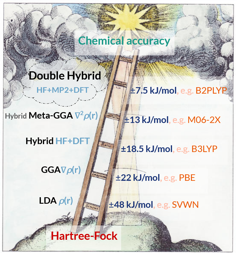
A schematic of the “rungs” of accuracy in the conceptual “Jacob’s ladder” organisation system of density functional methods. The qouted accuracy of each rung comes from a review by Goerigk & Grimme on density functional methods. Schematic of Jacob’s ladder modified from: Robert Fludd, Utriusque Cosmi, 1671, illustrated by Johann Theodor de Bry, Oppenheim and Frankfort.
Local density approximation (LDA) functionals use only the local electron density (\(\rho\)), generalised gradient approximation (GGA) functionals incorporate the electron density gradient (\(\nabla\rho\)), and meta-GGA functionals incorporate the second derivative or kinetic energy of the electron density (\(\nabla^2\rho\)). Improved accuracy relative to pure DFT functionals can be achieved by mixing in a component of a wavefunction method. When HF exchange is incorporated into DFT it is known as a “hybrid” method, and addition of a perturbative MP2-like correction yields a “double-hybrid” method. The RI approximation can be used for the MP2-like correction in double-hybrid methods. DFT methods, being formulated upon local electron densities, do not properly capture dispersion interactions and so are frequently combined with empirical dispersion corrections.
Global hybrid functionals
Pure DFT functionals suffer from self-interaction error (SIE), where the Coulomb repulsion of an electron with itself is non-zero due to the form of the exchange functional. The Slater determinant adopted for the HF exchange energy (\(E_{x}^{\mathrm{HF}}\)) exactly cancels SIE, and so SIE is lessened in hybrid functionals. Global hybrid (GH) functionals use a set fraction of HF exchange and have the form: \[E_{xc}^{\mathrm{GH}} = (1 - a_{x})E_{x}^{\mathrm{DFT}} + a_{x}E_{x}^{\mathrm{HF}} + E_{c}^{\mathrm{DFT}}\]
As an example, in the popular B3LYP method \(E_{c}^{\mathrm{DFT}}\) is calculated with the Lee, Yang, and Par (LYP) correlation functional, \(E_{x}^{\mathrm{DFT}}\) with the Becke88 (B88) exchange functional, and the HF exchange mixing coefficient, \(a_{x}\), is 0.2 at all distances.
Double-hybrid functionals
Double-hybrid density functionals (DHDFs) supplement \(E_{xc}[\rho]\) with a mixture of both non-local exchange and correlation energy from wavefunction methods, allowing them to recover more dynamic correlation and dispersion energy. DHDFs have the form: \[E_{xc}^{\mathrm{DHDF}} = (1 - a_{x})E_{x}^{\mathrm{DFT}} + a_{x}E_{x}^{\mathrm{HF}} + (1 - a_{c})E_{c}^{\mathrm{DFT}} + a_{c}E_{c}^{\mathrm{PT2}}\]
One of the first DHDFs was B2-PLYP which uses the same B88 and LYP functionals as B3LYP, and wavefunction mixing coefficients \(a_{x} = 0.47\) and \(a_{c} = 0.27\). The wavefunction mixing coefficients were re-optimised for specific chemical applications for the B2\(X\)-PLYP set of DHDFs. In a systematic survey by Karton et al. the “general-purpose” B2GP-PLYP functional, with \(a_{x} = 0.65\) and \(a_{c} = 0.36\), was found to be the most robust of the B2\(X\)-PLYP set methods, with maximum errors below 8 kJ/mol across all benchmark datasets surveyed.
Range separated functionals
The use of a single \(a_{x}\) mixing coefficient in GH functionals leads to incorrect behaviour at long-range electron-electron distances, resulting in poor accuracy for charge-transfer excitations. In range separated hybrids (RSHs) \(\alpha\) and \(\beta\) parameters are introduced to the exchange functional form, to smoothly connect between GH exchange at short range and exact HF exchange at long range: \[E_{x}^{\mathrm{RSH}} = (1 - \alpha)E_{x}^{\mathrm{DFT}} + \alpha E_{x}^{\mathrm{HF}} + \beta E_{x,\mu}^{\mathrm{HF}} - \beta E_{x,\mu}^{\mathrm{DFT}}\]
The value of \(\mu\) in a RSH functional determines how rapid the switch is between short range and long range exchange behaviour. For example, the CAM-B3LYP functional uses 0.19 \(E_{x}^{\mathrm{HF}}\) + 0.81 \(E_{x}^{\mathrm{B88}}\) at short-range but transitions to 0.65 \(E_{x}^{\mathrm{HF}}\) + 0.35 \(E_{x}^{\mathrm{B88}}\) at long-range.
I can provide a post on basis sets later, but the nomenclature in the field is messy. Best to go straight to the Basis Set Exchange